a function to model curve of a dataset using a local regression

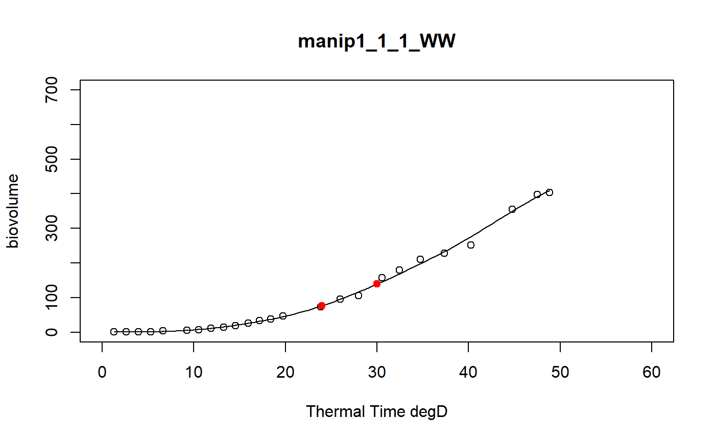
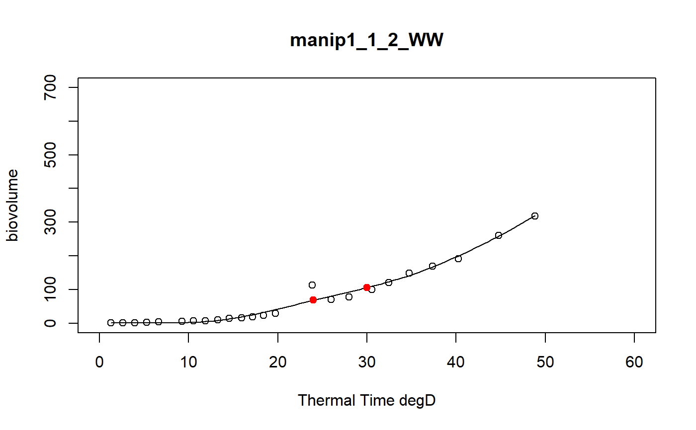
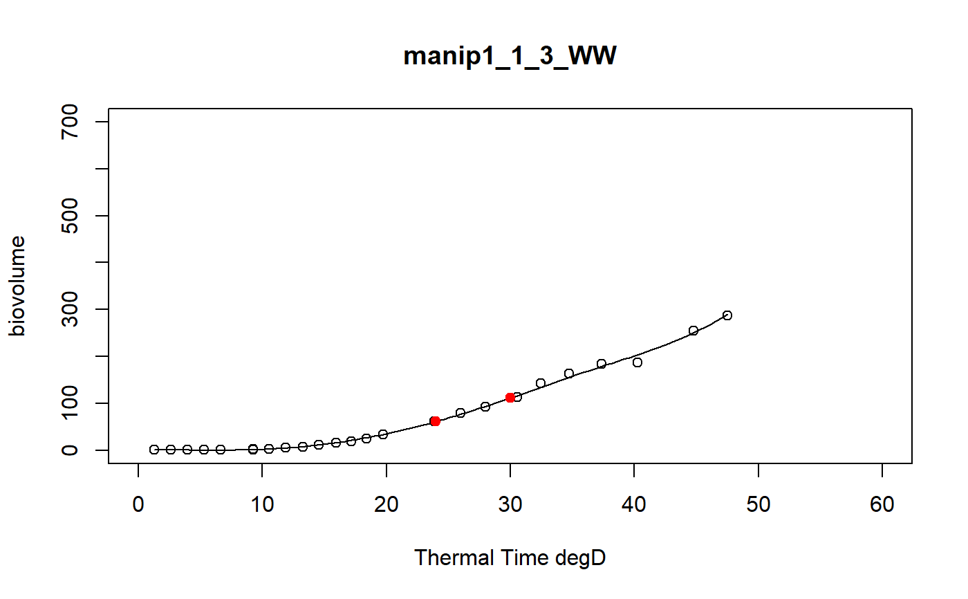
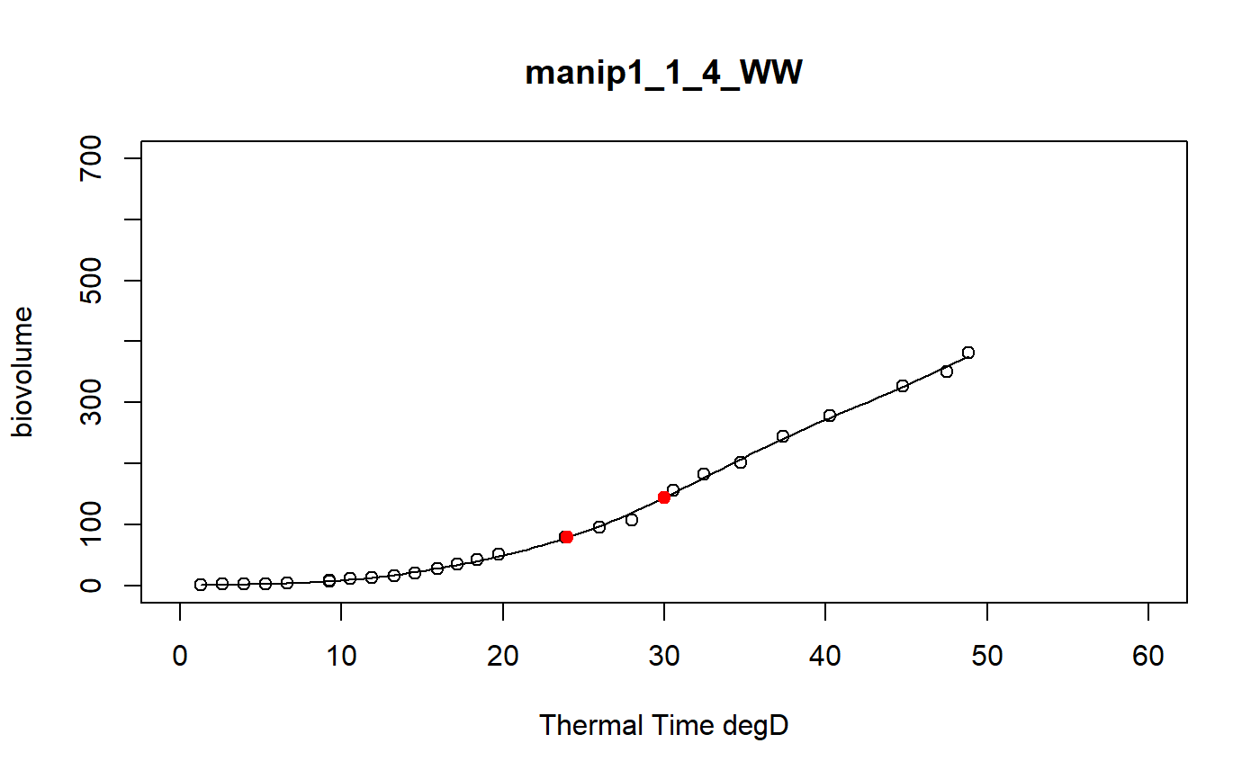
this function models each curve of a dataset using a local regression on biovolume, plant height or leaf area trait and extracts predictions at specific thermal times

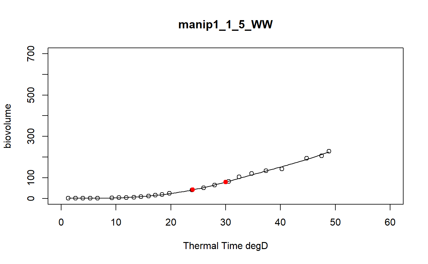
fitLocfit(datain, trait, xtime, myylim, tt, reference, myxlab)

Arguments

datain	input dataframe
trait	character, trait of interest to model (example biovolume, PH ...)
xtime	character, name of the thermal time column in the input dataset (example thermaltime)
myylim	numeric, max value of y-axis , varies according to trait
tt	numeric vector of thermal times at which predictions are recovered
reference	character, a column name indicating an unique identifiant of plant in the input dataset (example: Ref == concatenation of experimentAlias-Line-Position-scenario)
myxlab	character, a x label for the output graphics

Value

a dataframe of the predictions at tt thermal times for each plant of the input data set and the graphics of the smoothing curves

Details

the input dataset must contain a thermalTime column (numeric data) and a Ref column (unique id)

Examples

# \donttest{
# Take a while...
 myThermalTimes<-c(24,30)
selec<-c("manip1_1_1_WW","manip1_1_2_WW","manip1_1_3_WW",
         "manip1_1_4_WW","manip1_1_5_WW")
mydata<-plant1[plant1[,"Ref"] %in% selec,]
 resu<-fitLocfit(datain=mydata,trait="biovolume",xtime="thermalTime",
                 myylim=700,tt=myThermalTimes,reference="Ref",
                 myxlab="Thermal Time degD")
 str(resu)
#> 'data.frame':	10 obs. of  3 variables:
#>  $ Ref  : chr  "manip1_1_1_WW" "manip1_1_1_WW" "manip1_1_2_WW" "manip1_1_2_WW" ...
#>  $ xpred: num  24 30 24 30 24 30 24 30 24 30
#>  $ ypred: num  76.5 139.2 68.2 105.9 61.3 ...
# }