Phenoarch platform - Cleaning procedure - Curve level using SpATS
I.Sanchez
septembre 04, 2020
detectOutlierCurves.RmdObjective
This vignette deals with the detection of outlier plants in a lattice experiment using a spatial model using splines (SpATS library) [3]. Here the following steps of this procedure developed for Maize experiment but easily adaptable to others species:
- From a temporal dataset designed as plant1 with biomass (or biovolume) and plant height phenotypes. Extract predictions of these two phenotypes at a specific time point (for example just before the treatment) and create a dataset designed as plant4. Here, we will use the biomass and plant height predicted at 24 days at 20°C.
- From a temporal dataset of count of number of leaves, extract the phyllocron (slope of linear regression for each plant)
We so have a dataset with one row for each plant in the experiment containing the three phenotypes: biomass24, PH24 and Phy.
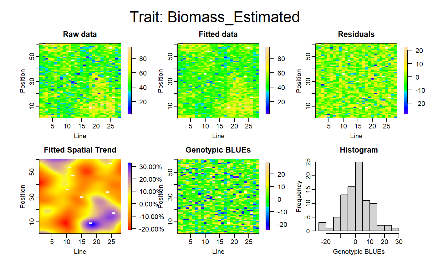
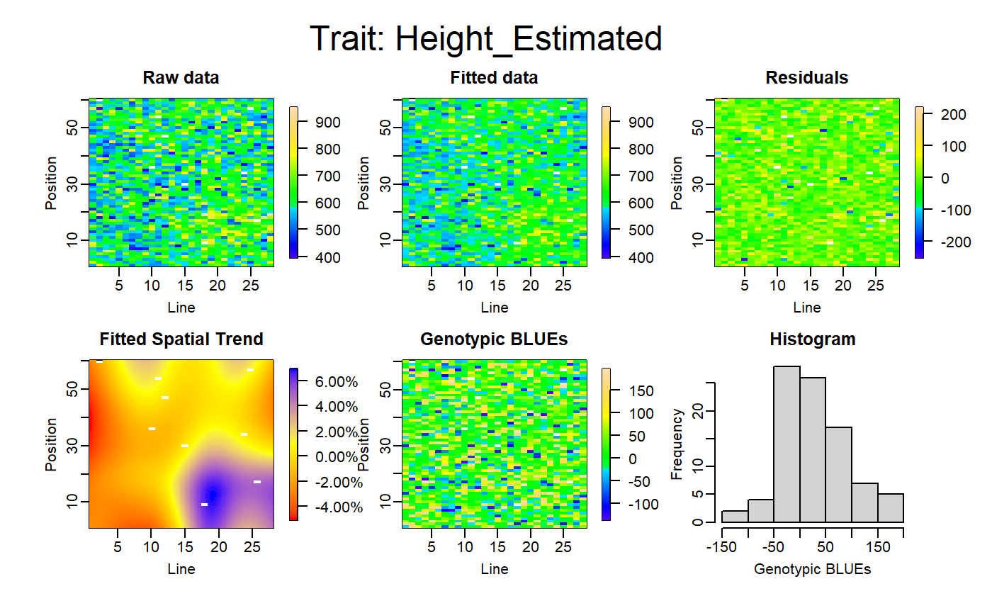
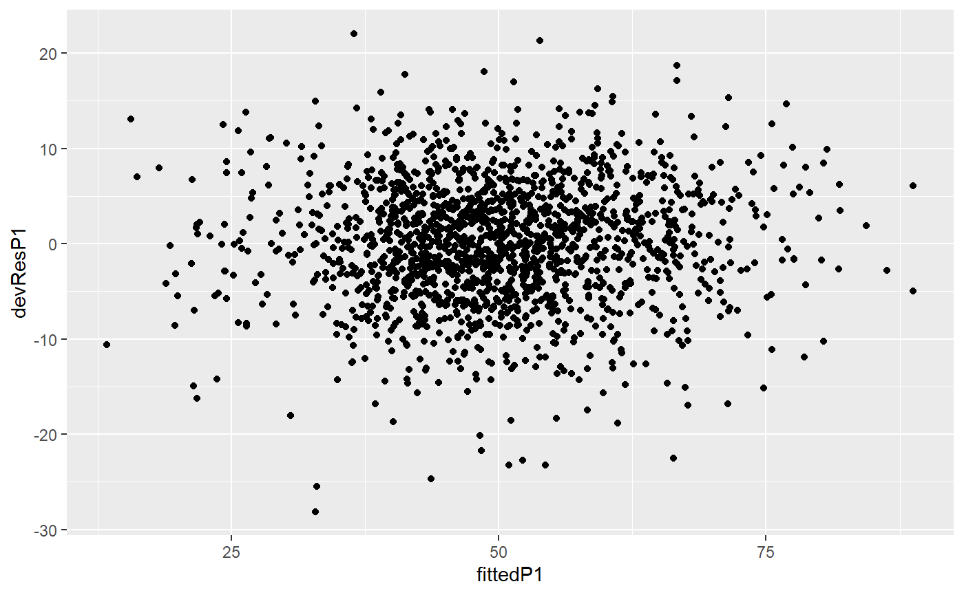
Apply a SpATS model on each phenotype, check the diagnostic graphics and retrieve the deviance residuals calculated by the model.
On the residuals, we can detect outlier plant(s) with a combined physiological criterion applying the following rules:
-
raw procedure: at a threshold=0.95 (can be modified)
- small plants are identified if \(res_i < \mu_{res} - qnorm(threshold) \times sd_{res}\) for biomass AND phyllocron
- big plants are identified if \(res_i > \mu_{res} + qnorm(threshold) \times sd_{res}\) for biomass AND plant height
Use the FuncDetectOutlierPlanMaize() and plotDetectOutlierPlantMaize() functions to do the previous steps.
Import of data
In this vignette, we use a toy data set of the openSilexStatR library (anonymized real data set).
This data set was obtained from an experiment of maize performed in the Phenoarch greenhouse composed of a conveyor belt structure of 28 lanes carrying 60 carts with one pot each (i.e. 1680 pots) (Cabrera-Bosquet et al. 2016). The data contains one experiment with 90 genotypes (Genotype) from two genotypic panels (Population) and two water scenarios (Treatment): well watered (WW) and water deficit (WD).
The leaf area and the biomass of individual plants are estimated from images taken in 13 directions. Briefly, pixels extracted from RGB images are converted into biomass and leaf area using linear models derived from regression of data from multiple side view images and destructive measurements performed at different phenological stages, from 5 to 14 appeared leaves (i.e. from 15 to 50 days at 20°C after emergence). Time courses of biomass (Biomass_Estimated) and leaf area (LA_Estimated) are expressed as a function of thermal time (TT). The height of each plants (Height_Estimated) is also estimated from the pictures. The number of visible leaves (count_leaf) is counted at least once a week on each plant. To prevent errors in leaf counting, leaves 5 and 10 of each plant are marked soon after appearance. The phyllocron is calculated as the slope of the linear regression bewtween the number of leaves and the thermal time at 2017-04-27 day, before the beginning of the water deficit. The unique ID of the plant is recorded (plantId), together with the pot position in row (Row) and in column (Col).
  mydata<-PAdata
  str(mydata)
## 'data.frame':    55799 obs. of  13 variables:
##  $ Time             : Factor w/ 72 levels "2017-04-13","2017-04-14",..: 2 3 4 5 6 7 8 9 10 11 ...
##  $ plantId          : Factor w/ 1671 levels "01_01","01_02",..: 1 1 1 1 1 1 1 1 1 1 ...
##  $ Genotype         : Factor w/ 90 levels "GenoA1","GenoA10",..: 39 39 39 39 39 39 39 39 39 39 ...
##  $ Treatment        : Factor w/ 2 levels "WD","WW": 1 1 1 1 1 1 1 1 1 1 ...
##  $ Population       : Factor w/ 2 levels "Panel1","Panel2": 1 1 1 1 1 1 1 1 1 1 ...
##  $ Row              : int  1 1 1 1 1 1 1 1 1 1 ...
##  $ Col              : int  1 1 1 1 1 1 1 1 1 1 ...
##  $ Biomass_Estimated: num  NA NA NA NA 1.85 ...
##  $ LA_Estimated     : num  0.00398 0.00555 0.00742 0.01089 0.01299 ...
##  $ Height_Estimated : num  120 173 242 266 249 ...
##  $ count_leaf       : num  4.2 NA NA NA NA 6.2 NA NA NA NA ...
##  $ phyllocron       : num  NA NA NA NA NA NA NA NA NA NA ...
##  $ TT               : int  104 NA NA NA NA 109 NA NA NA NA ...
SpATS library
Detection of outliers
test<-FuncDetectOutlierPlantMaize(datain=mydata,dateBeforeTrt="2017-04-27",
                param1="Biomass_Estimated",param2="Height_Estimated",
                param3="phyllocron",paramGeno="Genotype",
                paramCol="Col",paramRow="Row",
                threshold=0.95,nCol=28,nRow=60,genotype.as.random=FALSE,
                timeColumn = "Time")
The FuncDetectOutlierPlantMaize() returns a list of 6 elements :
- outputDataframe: a dataframe with the used data set, the fitted values and residuals calculated by the models, the plants flagged as outlier
- smallOutlier: a data.frame of the small plants detected as outliers
- bigOutlier: a data.frame of the big plants detected as outliers
- m1: A list of the SpATS results for param1
- m2: A list of the SpATS results for param2
- m3: A list of the SpATS results for param3

Dataset highlighting the outlier plants
test$smallOutlier
##          Time plantId Genotype Treatment Population Position Line
## 1  2017-04-27   05_03   GenoA6        WW     Panel1        3    5
## 2  2017-04-27   06_57  GenoA57        WW     Panel1       57    6
## 3  2017-04-27   07_02   GenoB7        WD     Panel2        2    7
## 4  2017-04-27   07_18  GenoB11        WD     Panel2       18    7
## 5  2017-04-27   09_57   GenoB3        WD     Panel2       57    9
## 6  2017-04-27   12_50  GenoA30        WD     Panel1       50   12
## 7  2017-04-27   13_28  GenoA27        WD     Panel1       28   13
## 8  2017-04-27   13_30  GenoA42        WD     Panel1       30   13
## 9  2017-04-27   14_36  GenoA17        WW     Panel1       36   14
## 10 2017-04-27   17_49  GenoB20        WD     Panel2       49   17
## 11 2017-04-27   18_15  GenoA22        WW     Panel1       15   18
## 12 2017-04-27   18_41  GenoA20        WW     Panel1       41   18
## 13 2017-04-27   21_43  GenoA18        WD     Panel1       43   21
## 14 2017-04-27   22_56   GenoA7        WW     Panel1       56   22
## 15 2017-04-27   25_42  GenoA29        WW     Panel1       42   25
## 16 2017-04-27   27_48  GenoB23        WW     Panel2       48   27
## 17 2017-04-27   28_01  GenoA45        WD     Panel1        1   28
## 18 2017-04-27   28_37  GenoA29        WD     Panel1       37   28
##    Biomass_Estimated LA_Estimated Height_Estimated count_leaf phyllocron TT  R
## 1          19.053046   0.04054923         496.8150         NA  0.2866803 NA  5
## 2          26.710540   0.04348831         682.7700         NA  0.3491393 NA  6
## 3          31.545385   0.05775239         597.6300         NA  0.2395393 NA  7
## 4          23.917150   0.04065245         476.4375         NA  0.2637236 NA  7
## 5          44.095749   0.06336016         506.3025         NA  0.2977607 NA  9
## 6          41.800552   0.06643003         694.5675         NA  0.2981148 NA 12
## 7           9.439104   0.02706301         575.1075         NA  0.2605263 NA 13
## 8          29.777812   0.04720002         741.7988         NA  0.2596730 NA 13
## 9           6.538781   0.02208032         481.1400         NA  0.2058197 NA 14
## 10          2.735184   0.02487973         478.2113         NA  0.2364853 NA 17
## 11         40.809394   0.05455394         733.8375         NA  0.3296840 NA 18
## 12         38.077743   0.05350347         567.1463         NA  0.3233634 NA 18
## 13         29.502695   0.04313317         525.4425         NA  0.2540708 NA 21
## 14         49.972882   0.07000937         736.8900         NA  0.3138175 NA 22
## 15         28.169621   0.04284785         492.7725         NA  0.3175074 NA 25
## 16         12.484720   0.03674674         551.2650         NA  0.2558459 NA 27
## 17         21.620858   0.04142434         651.7500         NA  0.3087944 NA 28
## 18         33.709486   0.05006771         502.4250         NA  0.2940863 NA 28
##     C  devResP1    devResP2    devResP3 fittedP1 fittedP2  fittedP3
## 1   3 -24.65652 -252.051084 -0.03212489 43.70957 748.8661 0.3188052
## 2  57 -21.68928   58.741134 -0.03576921 48.39982 624.0289 0.3849086
## 3   2 -15.53607   36.153866 -0.04149007 47.08145 561.4761 0.2810294
## 4  18 -12.41711  -57.000785 -0.03814611 36.33426 533.4383 0.3018697
## 5  57 -15.65752   10.851758 -0.02536935 59.75327 495.4507 0.3231301
## 6  50 -13.64368   18.574363 -0.02539854 55.44423 675.9931 0.3235133
## 7  28 -14.22699  -49.386121 -0.03700164 23.66609 624.4936 0.2975280
## 8  30 -14.61140   21.019183 -0.03084497 44.38921 720.7796 0.2905180
## 9  36 -14.94456 -124.456121 -0.06904976 21.48334 605.5961 0.2748694
## 10 49 -10.63955 -196.665692 -0.02631130 13.37473 674.8769 0.2627966
## 11 15 -17.47116   -1.654703 -0.03217222 58.28055 735.4922 0.3618562
## 12 41 -13.12194  -23.986932 -0.02567852 51.19968 591.1332 0.3490420
## 13 43 -22.76087  -82.890463 -0.04273011 52.26356 608.3330 0.2968009
## 14 56 -12.65982  -21.910579 -0.02585889 62.63271 758.8006 0.3396764
## 15 42 -20.10408 -117.653029 -0.03311315 48.27370 610.4255 0.3506206
## 16 48 -18.03684 -100.787582 -0.03660976 30.52156 652.0526 0.2924556
## 17  1 -16.82632  -14.777683 -0.02389344 38.44717 666.5277 0.3326879
## 18 37 -14.21707  -93.058262 -0.02837121 47.92656 595.4833 0.3224575
##      mean.devP1 sd.devP1    mean.devP2 sd.devP2   mean.devP3   sd.devP3
## 1  1.240996e-14 6.413921 -1.621669e-13 44.29345 3.794596e-16 0.01446087
## 2  1.240996e-14 6.413921 -1.621669e-13 44.29345 3.794596e-16 0.01446087
## 3  1.240996e-14 6.413921 -1.621669e-13 44.29345 3.794596e-16 0.01446087
## 4  1.240996e-14 6.413921 -1.621669e-13 44.29345 3.794596e-16 0.01446087
## 5  1.240996e-14 6.413921 -1.621669e-13 44.29345 3.794596e-16 0.01446087
## 6  1.240996e-14 6.413921 -1.621669e-13 44.29345 3.794596e-16 0.01446087
## 7  1.240996e-14 6.413921 -1.621669e-13 44.29345 3.794596e-16 0.01446087
## 8  1.240996e-14 6.413921 -1.621669e-13 44.29345 3.794596e-16 0.01446087
## 9  1.240996e-14 6.413921 -1.621669e-13 44.29345 3.794596e-16 0.01446087
## 10 1.240996e-14 6.413921 -1.621669e-13 44.29345 3.794596e-16 0.01446087
## 11 1.240996e-14 6.413921 -1.621669e-13 44.29345 3.794596e-16 0.01446087
## 12 1.240996e-14 6.413921 -1.621669e-13 44.29345 3.794596e-16 0.01446087
## 13 1.240996e-14 6.413921 -1.621669e-13 44.29345 3.794596e-16 0.01446087
## 14 1.240996e-14 6.413921 -1.621669e-13 44.29345 3.794596e-16 0.01446087
## 15 1.240996e-14 6.413921 -1.621669e-13 44.29345 3.794596e-16 0.01446087
## 16 1.240996e-14 6.413921 -1.621669e-13 44.29345 3.794596e-16 0.01446087
## 17 1.240996e-14 6.413921 -1.621669e-13 44.29345 3.794596e-16 0.01446087
## 18 1.240996e-14 6.413921 -1.621669e-13 44.29345 3.794596e-16 0.01446087
##    lower.devP1 lower.devP2 lower.devP3 upper.devP1 upper.devP2 upper.devP3
## 1    -10.54996   -72.85624 -0.02378602    10.54996    72.85624  0.02378602
## 2    -10.54996   -72.85624 -0.02378602    10.54996    72.85624  0.02378602
## 3    -10.54996   -72.85624 -0.02378602    10.54996    72.85624  0.02378602
## 4    -10.54996   -72.85624 -0.02378602    10.54996    72.85624  0.02378602
## 5    -10.54996   -72.85624 -0.02378602    10.54996    72.85624  0.02378602
## 6    -10.54996   -72.85624 -0.02378602    10.54996    72.85624  0.02378602
## 7    -10.54996   -72.85624 -0.02378602    10.54996    72.85624  0.02378602
## 8    -10.54996   -72.85624 -0.02378602    10.54996    72.85624  0.02378602
## 9    -10.54996   -72.85624 -0.02378602    10.54996    72.85624  0.02378602
## 10   -10.54996   -72.85624 -0.02378602    10.54996    72.85624  0.02378602
## 11   -10.54996   -72.85624 -0.02378602    10.54996    72.85624  0.02378602
## 12   -10.54996   -72.85624 -0.02378602    10.54996    72.85624  0.02378602
## 13   -10.54996   -72.85624 -0.02378602    10.54996    72.85624  0.02378602
## 14   -10.54996   -72.85624 -0.02378602    10.54996    72.85624  0.02378602
## 15   -10.54996   -72.85624 -0.02378602    10.54996    72.85624  0.02378602
## 16   -10.54996   -72.85624 -0.02378602    10.54996    72.85624  0.02378602
## 17   -10.54996   -72.85624 -0.02378602    10.54996    72.85624  0.02378602
## 18   -10.54996   -72.85624 -0.02378602    10.54996    72.85624  0.02378602
##    lower.spatsP1 lower.spatsP2 lower.spatsP3 upper.spatsP1 upper.spatsP2
## 1              0             0             0             1             1
## 2              0             1             0             1             1
## 3              0             1             0             1             1
## 4              0             1             0             1             1
## 5              0             1             0             1             1
## 6              0             1             0             1             1
## 7              0             1             0             1             1
## 8              0             1             0             1             1
## 9              0             0             0             1             1
## 10             0             0             0             1             1
## 11             0             1             0             1             1
## 12             0             1             0             1             1
## 13             0             0             0             1             1
## 14             0             1             0             1             1
## 15             0             0             0             1             1
## 16             0             0             0             1             1
## 17             0             1             0             1             1
## 18             0             0             0             1             1
##    upper.spatsP3 flagLowerSpats flagUpperSpats
## 1              1              0              1
## 2              1              0              1
## 3              1              0              1
## 4              1              0              1
## 5              1              0              1
## 6              1              0              1
## 7              1              0              1
## 8              1              0              1
## 9              1              0              1
## 10             1              0              1
## 11             1              0              1
## 12             1              0              1
## 13             1              0              1
## 14             1              0              1
## 15             1              0              1
## 16             1              0              1
## 17             1              0              1
## 18 1 0 1test$bigOutlier
##         Time plantId Genotype Treatment Population Position Line
## 1 2017-04-27   07_55   GenoB3        WW     Panel2       55    7
## 2 2017-04-27   11_29  GenoA36        WW     Panel1       29   11
## 3 2017-04-27   17_17  GenoB24        WW     Panel2       17   17
##   Biomass_Estimated LA_Estimated Height_Estimated count_leaf phyllocron TT  R
## 1          71.41276   0.09273917         569.7450         NA  0.3697377 NA  7
## 2          36.67895   0.06258974         704.2200         NA  0.3088115 NA 11
## 3          58.48472   0.07994443         769.4362         NA  0.3232828 NA 17
##    C devResP1 devResP2   devResP3 fittedP1 fittedP2  fittedP3   mean.devP1
## 1 55 13.80518 76.96394 0.03304748 57.60759 492.7811 0.3366902 1.240996e-14
## 2 29 12.46516 78.23241 0.01048244 24.21379 625.9876 0.2983290 1.240996e-14
## 3 17 22.03344 73.26826 0.03389641 36.45128 696.1680 0.2893864 1.240996e-14
##   sd.devP1    mean.devP2 sd.devP2   mean.devP3   sd.devP3 lower.devP1
## 1 6.413921 -1.621669e-13 44.29345 3.794596e-16 0.01446087   -10.54996
## 2 6.413921 -1.621669e-13 44.29345 3.794596e-16 0.01446087   -10.54996
## 3 6.413921 -1.621669e-13 44.29345 3.794596e-16 0.01446087   -10.54996
##   lower.devP2 lower.devP3 upper.devP1 upper.devP2 upper.devP3 lower.spatsP1
## 1   -72.85624 -0.02378602    10.54996    72.85624  0.02378602             1
## 2   -72.85624 -0.02378602    10.54996    72.85624  0.02378602             1
## 3   -72.85624 -0.02378602    10.54996    72.85624  0.02378602             1
##   lower.spatsP2 lower.spatsP3 upper.spatsP1 upper.spatsP2 upper.spatsP3
## 1             1             1             0             0             0
## 2             1             1             0             0             1
## 3             1             1             0             0             0
##   flagLowerSpats flagUpperSpats
## 1              1              0
## 2              1              0
## 3              1              0
The user can save the residuals and detected outliers in an output file, using write.table() function.
Plots
plotDetectOutlierPlantMaize(datain=PAdata,
                            outmodels=test$smallOutlier,
                            x="Time",
                            y="Biomass_Estimated",
                            genotype="Genotype",
                            idColor="Treatment",
                            idFill="plantId")
## Warning: Removed 1968 rows containing missing values (geom_point).## Warning: Removed 122 rows containing missing values (geom_point).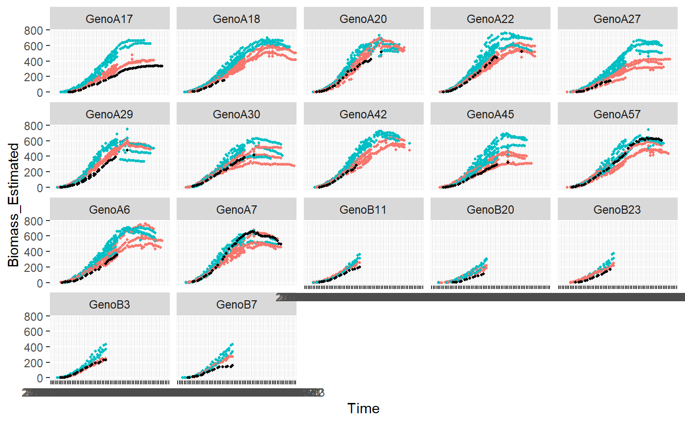
plotDetectOutlierPlantMaize(datain=PAdata,
                            outmodels=test$bigOutlier,
                            x="Time",
                            y="Biomass_Estimated",
                            genotype="Genotype",
                            idColor="Treatment",
                            idFill="plantId")
## Warning: Removed 280 rows containing missing values (geom_point).## Warning: Removed 16 rows containing missing values (geom_point).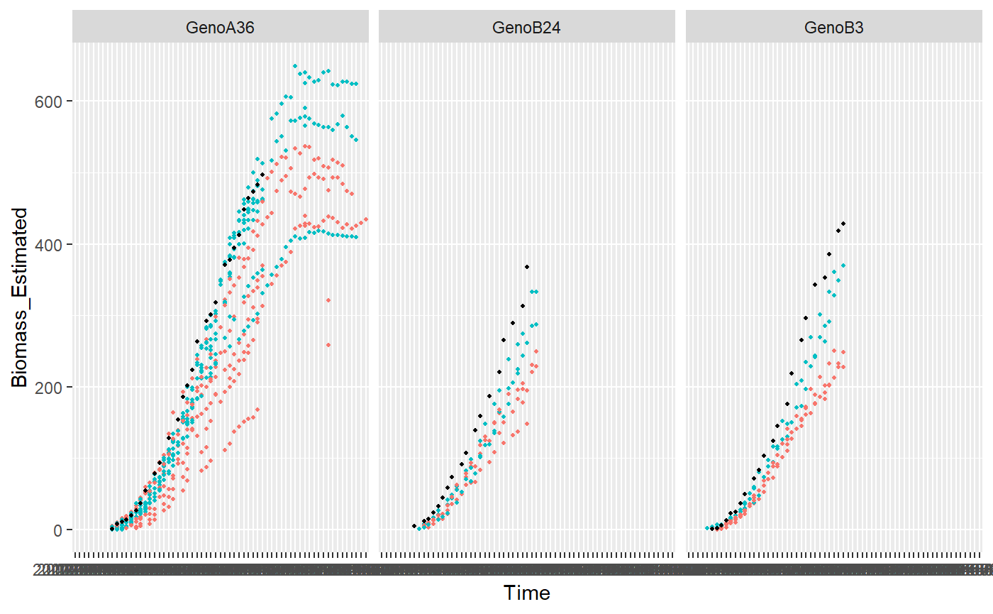
Session info
## R version 4.0.2 (2020-06-22)
## Platform: x86_64-w64-mingw32/x64 (64-bit)
## Running under: Windows 10 x64 (build 18363)
##
## Matrix products: default
##
## locale:
## [1] LC_COLLATE=French_France.1252  LC_CTYPE=French_France.1252
## [3] LC_MONETARY=French_France.1252 LC_NUMERIC=C
## [5] LC_TIME=French_France.1252
##
## attached base packages:
## [1] stats     graphics  grDevices utils     datasets  methods   base
##
## other attached packages:
## [1] ggplot2_3.3.2        openSilexStatR_1.1.0 tidyr_1.1.2
## [4] dplyr_1.0.2
##
## loaded via a namespace (and not attached):
##  [1] maps_3.3.0         splines_4.0.2      dotCall64_1.0-0    gtools_3.8.2
##  [5] assertthat_0.2.1   expm_0.999-5       CARBayesdata_2.2   sp_1.4-2
##  [9] stats4_4.0.2       yaml_2.2.1         LearnBayes_2.15.1  truncdist_1.0-2
## [13] pillar_1.4.6       backports_1.1.9    lattice_0.20-41    glue_1.4.2
## [17] digest_0.6.25      RColorBrewer_1.1-2 colorspace_1.4-1   plyr_1.8.6
## [21] htmltools_0.5.0    Matrix_1.2-18      pkgconfig_2.0.3    raster_3.3-13
## [25] CARBayesST_3.1     gmodels_2.18.1     purrr_0.3.4        scales_1.1.1
## [29] gdata_2.18.0       tibble_3.0.3       farver_2.0.3       generics_0.0.2
## [33] ellipsis_0.3.1     withr_2.2.0        magrittr_1.5       crayon_1.3.4
## [37] deldir_0.1-28      memoise_1.1.0      evaluate_0.14      GGally_2.0.0
## [41] fs_1.4.2           nlme_3.1-148       MASS_7.3-51.6      foreign_0.8-80
## [45] truncnorm_1.0-8    class_7.3-17       data.table_1.13.0  tools_4.0.2
## [49] shapefiles_0.7     lifecycle_0.2.0    matrixStats_0.56.0 stringr_1.4.0
## [53] munsell_0.5.0      compiler_4.0.2     pkgdown_1.5.1      e1071_1.7-3
## [57] evd_2.3-3          rlang_0.4.7        classInt_0.4-3     units_0.6-7
## [61] grid_4.0.2         rstudioapi_0.11    htmlwidgets_1.5.1  spam_2.5-1
## [65] crosstalk_1.1.0.1  labeling_0.3       rmarkdown_2.3      SpATS_1.0-11
## [69] boot_1.3-25        testthat_2.3.2     gtable_0.3.0       codetools_0.2-16
## [73] reshape_0.8.8      DBI_1.1.0          R6_2.4.1           lubridate_1.7.9
## [77] gridExtra_2.3      knitr_1.29         rgdal_1.5-16       rprojroot_1.3-2
## [81] spdep_1.1-5        KernSmooth_2.23-17 desc_1.2.0         matrixcalc_1.0-3
## [85] stringi_1.4.6      Rcpp_1.0.5         fields_11.4        vctrs_0.3.4
## [89] sf_0.9-5           leaflet_2.0.3      spData_0.3.8       tidyselect_1.1.0
## [93] xfun_0.16          coda_0.19-3
References
- R Development Core Team (2015). R: A language and environment for statistical computing. R Foundation for Statistical Computing, Vienna, Austria. ISBN 3-900051-07-0, URL http://www.R-project.org.
- Maria Xose Rodriguez-Alvarez, Martin P. Boer, Fred A. van Eeuwijk, Paul H.C. Eilers (2017). Correcting for spatial heterogeneity in plant breeding experiments with P-splines. Spatial Statistics URL https://doi.org/10.1016/j.spasta.2017.10.003
- Alvarez Prado, S., Sanchez, I., Cabrera Bosquet, L., Grau, A., Welcker, C., Tardieu, F., Hilgert, N. (2019). To clean or not to clean phenotypic datasets for outlier plants in genetic analyses?. Journal of Experimental Botany, 70 (15), 3693-3698. , DOI : 10.1093/jxb/erz191 https://prodinra.inra.fr/record/481355